3 Truncated Triangular Distribution
3.1 Truncated Distribution
A truncated distribution, simply put, is a distribution derived from another such that it’s domain is restricted to some interval \(]a,b]\). The function itself might not change but because we require the area under the PDF to be equal to 1, a transformation is due. One of the strengths of this distribution lies in the fact that most of it properties can be calculated from methods already implemented in the underlying distribution, meaning that the functions and values need not be derived analytically and so it’s implementation is easily generalized.
3.2 Truncated Triangular PDF
Since we’re handling more than one distribution, let’s distinguish them symbolically.
Let \(Y\sim f(y) = Triangular(L, U, M)\) and \(X\sim f(x|a < X \leq b) = h(x)\)
The truncated distribution has the following PDF, regardless of the underlying distribution.
\[ h(x)= \begin{cases} \frac{f(x)}{F(b)-F(a)}\quad&(a< x\leq b)\\ 0\quad&(x\ \notin\ ]a,b])\\ \end{cases} \]
Multiplying the original distribution’s PDF by a factor of \(\frac{1}{F(b)-F(a)}\) just scales it so the area removed by truncating the domain gets compensated for. Because we can already account for \(f(x)\) and \(F(x)\) in our original implementation of the triangular distribution, there is no need to analyticaly derive the new PDF. Let’s store an instance of the triangular distribution list in a variable and call it’s functions and values on demand.
## Create a list that contains the major properties of a triangular distribution with L = 2, U = 9, and M = 7
triangular.distribution <- generate.triangular(L = 2, U = 9, M = 7)
We will use this triangular as the distribution to truncate
truncated.distribution <- function(x, a, b) {
  if (a < x & x <= b) {
    pdf.g <- triangular.distribution$pdf
    cumul.F <- triangular.distribution$cdf
    result <- pdf.g(x) / (cumul.F(b) - cumul.F(a))
    return(result)
  } else {
    result <- 0
    return(result)
  }
}
This function takes some x and evaluates the truncated triangular PDF defined in the triangular.distribution variable.
Because of the nature of the plot.function() method, we must make our function compatible with vectors, meaning that passing a vector as its x parameter would apply the function to every element in it. Notice the .... This just means that any subsequent parameters get passed to the underlying truncated.distribution() function.
plot.function(
  function(x) {truncated.distribution.vectorized(x, 2, 9)},
  from = 2,
  to = 9,
  main = "Truncated Triangular Distributions",
  ylab = "f(x)",
  ylim = c(0, 0.5)
)

## Additional plots get included in the first rather than into a new canvas
## when the `add` parameter is set to TRUE.
plot.function(
  function(x) {truncated.distribution.vectorized(x, 3, 8)},
  from = 2,
  to = 9,
  col = "red",
  add = TRUE
)

plot.function(
  function(x) {truncated.distribution.vectorized(x, 4, 7)},
  from = 2,
  to = 9,
  col = "blue",
  add = TRUE
)

## Let's also include a legend so we can distinguish all three distributions.
legend(
  x = 2,
  y = 0.5,
  legend = c("f(x|2 < x <= 9)", "f(x|3 < x <= 8)", "f(x|4 < x <= 7)"),
  col = c("black", "red", "blue"),
  lty = 1
)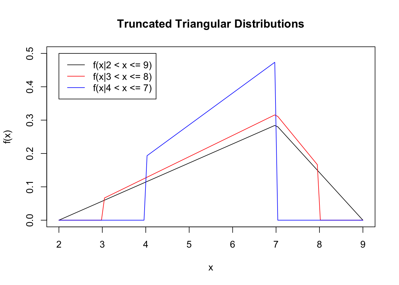
Notice how our distributions get scaled up further as the new domain becomes narrower. The black distribution faces no changes because cutting it’s domain to \(a=2\) and \(b=9\) makes no difference, and so the triangular distribution remains.
3.3 Truncated Triangular CDF
The CDF is quite straight forward to understand. Because the PDF of the runcated triangular is the same as the original only restricted in its domain and scaled by a constant factor of \(\frac{1}{F(b)-F(a)}\), all we really need to falculate \(H(x)\) is to calculate \(F(x)\), subtract the portion now unaccounted for by the restrictions to the domain (\(F(a)\)), and scale by the same factor as the PDF.
\[ H(x) = \begin{cases} 0 \quad& x\leq a\\ \frac{F(x)-F(a)}{F(b)-F(a)} \quad& a < x \leq b\\ 1 \quad& b < x \end{cases} \]
Again, the implementation of the triangular distribution already considers a function to calculate the triangular CDF, meaning that there is no need to analyticaly derive the equation. It’s good enough to call the CDF directly.
cumulative.truncated.distribution <- function(x, a, b) {
  if (x <= a) {
    result <- 0
  } else if (a < x & x <= b) {
    result <- (triangular.distribution$cdf(x) - triangular.distribution$cdf(a)) / (triangular.distribution$cdf(b) - triangular.distribution$cdf(a))
  } else if (x > b){
    result <- 1
  }
  return(result)
}

cumulative.truncated.distribution.vectorized <- function(x, ...) {
    sapply(x, cumulative.truncated.distribution, ...)
}
The code for the plots also shouldn’t change much. No change has been made to the parameters of each distribution.
plot.function(
  function(x) {cumulative.truncated.distribution.vectorized(x, 2, 9)},
  from = 0,
  to = 10,
  main = "Cumulative Truncated Triangular Distributions",
  ylab = "F(x)",
  ylim = c(0, 1)
)

plot.function(
  function(x) {cumulative.truncated.distribution.vectorized(x, 3, 8)},
  from = 0,
  to = 10,
  col = "red",
  add = TRUE
)

plot.function(
  function(x) {cumulative.truncated.distribution.vectorized(x, 4, 7)},
  from = 0,
  to = 10,
  col = "blue",
  add = TRUE
)

legend(
  x = 0,
  y = 1,
  legend = c("F(x|2 < x <= 9)", "F(x|3 < x <= 8)", "F(x|4 < x <= 7)"),
  col = c("black", "red", "blue"),
  lty = 1
)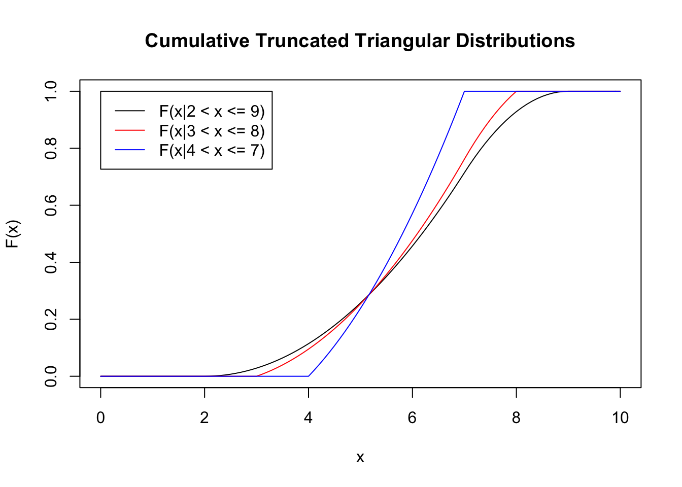
Notice how the cumulative distribution approaches one very quickly. This makes sense considering that, because of the bounds of the domain of the triangular distribution, \(X\) is guaranteed to be smaller than \(U\), at which point the probability is one.
3.4 Inverse Truncated Triangular CDF
What if we already had a probability in mind but wanted to find the matching \(x\)? Well, in that case, we would need to calculate an inverse CDF. Given some probability \(p\), what \(x\) delimits \(X\) such that \(p\) is \(P(X\leq x)\).
Or in other words, find \(g\) such that:
\[ g(p) = H^{-1}(p) = H^{-1}(H(x)) = x \]
Explicitly, we really just need to solve for \(x\) in the following equation.
\[ H(x)=\frac{F(x)-F(a)}{F(b)-F(a)}=p \]
The resulting expression will be in terms of a probability \(p\).
\[ H^{-1}(p) = F^{-1}\left(p(F(b)-F(a)) + F(a)\right) \]
Remember how our triangular.distribution object has cdf() and inverse.cdf() methods, meaning the inverse cdf of the truncated triangular distribution can also be computed from the implementation of the base distribution.
inverse.cumulative.truncated.distribution <- function(p, a, b) {
  result <- tringular.distribution$inverse.cdf(
    p * (tringular.distribution$cdf(b) - tringular.distribution$cdf(a))
    + tringular.distribution$cdf(a)
  )
  return(result)
}
No plots for this one considering how it just mirrors the regular CDF over the \(y=x\) line. Do consider, this distribution is only defined for \(p\in[0,1]\). Some error handling could benefit your code’s reliability.
3.5 Measures of Central Tendency and Spread
We do come across a challenge when trying to figure out expressions for these statistics. First we must derive their expression analytically because they can’t be expressed just in terms of what we have already implemented in the triangular distribution (We must evaluate definite integrals); second, because these definite integral explicitly make use of the underlying triangular distribution, they can’t be generalised to the whole family of truncated distributions; and finally, the triangular distribution is a piecewise function, meaning the procedure to derive an expression must be done on a case by case basis.
3.5.1 Mean
The expected value of a random variable \(X\).
\[ E(X) = \int_{-\infty}^{\infty}xh(x)dx = \int_{a}^{b}x\cdot\frac{f(x)}{F(b)-F(a)}dx= \frac{\int_{a}^{b}xf(x)dx}{F(b)-F(a)} \] Case 1 (\(L \leq a \leq b < M\)):
\[ E(X)=\frac{\int_{a}^{b} x \cdot \frac{2(x-L)}{(U-L)(M-L)} dx}{F(b)-F(a)} \]
\[ = \frac{\frac{2\left( b^{3} - a^{3} - 3L\left( \frac{b^{2}}{2} - \frac{a^{2}}{2} \right) \right)}{3(U-L)(M-L)}}{F(b)-F(a)} \]
Case 2 (\(L \leq a < M \leq b \leq U\)):
\[ E(X)=\frac{\int_{a}^{M} x \cdot \frac{2(x-L)}{(U-L)(M-L)} dx + \int_{M}^{b} x \cdot \frac{2(U-x)}{(U-L)(U-M)} dx}{F(b)-F(a)} \]
\[ = \frac{\frac{-M^3U-2a^3U+3La^2U+3Mb^2U-3Lb^2U+LM^3+2Ma^3-3LMa^2-2Mb^3+2Lb^3}{3(U-L)(M-L)(U-M)}}{F(b)-F(a)} \]
Case 3 (\(M \leq a \leq b \leq U\)):
\[ E(X)=\frac{\int_{M}^{b} x \cdot \frac{2(U-x)}{(U-L)(U-M)} dx}{F(b)-F(a)} \]
\[ = \frac{\frac{3b^2U-3M^2U-2b^3+2M^3}{3\left(U-L\right)\left(U-M\right)}}{F(b)-F(a)} \]
3.5.2 Median
Value \(x\) such that the probability that a random variable \(X\) be smaller is 0.5.
\[ \text{Median(X)} = H^{-1}(0.5) \]
This one is straight forward. We already implemented the inverse CDF.
3.5.3 Mode
Value of a random variable \(X\) for which \(f(x)\) is at its maximum. Once again, we rely on the cases and calculate the mode according to where the bounds of the truncated fall.
\[ \text{Mode(X)} = \begin{cases} b \quad& (L \leq a \leq b < M)\\ M \quad& (L \leq a < M \leq b \leq U)\\ a \quad& (M \leq a \leq b \leq U) \end{cases} \]
3.5.4 Variance
Measure of spread of the distribution with respect to the mean.
\[ \text{Var(X)} = \int_{-\infty}^{\infty}x^{2}h(x)dx - E(X)^{2} = \int_{a}^{b}x^{2}\cdot\frac{f(x)}{F(b)-F(a)}dx - E(X)^{2} = \frac{\int_{a}^{b}x^{2}f(x)dx}{F(b)-F(a)} - E(X)^{2} \]
Case 1 (\(L \leq a \leq b < M\)):
\[ \text{Var}(X)=\frac{\int_{a}^{b} x^{2} \cdot \frac{2(x-L)}{(U-L)(M-L)} dx}{F(b)-F(a)}-E(X)^{2} \]
\[ = \frac{\frac{-4L\left(\frac{b^3}{3}-\frac{a^3}{3}\right)+b^4-a^4}{2\left(U-L\right)\left(M-L\right)}}{F(b)-F(a)}-E(X)^{2} \]
Case 2 (\(L \leq a < M \leq b \leq U\)):
\[ \text{Var}(X)=\frac{\int_{a}^{M} x^{2} \cdot \frac{2(x-L)}{(U-L)(M-L)} dx + \int_{M}^{b} x^{2} \cdot \frac{2(U-x)}{(U-L)(U-M)} dx}{F(b)-F(a)}-E(X)^{2} \]
\[ = \frac{\frac{-M^4U-3a^4U+4La^3U+4Mb^3U-4Lb^3U+LM^4+3Ma^4-4LMa^3-3Mb^4+3Lb^4}{6\left(U-L\right)\left(M-L\right)\left(U-M\right)}}{F(b)-F(a)}-E(X)^{2} \]
Case 3 (\(M \leq a \leq b \leq U\)):
\[ \text{Var}(X)=\frac{\int_{M}^{b} x^{2} \cdot \frac{2(U-x)}{(U-L)(U-M)} dx}{F(b)-F(a)}-E(X)^{2} \]
\[ = \frac{\frac{4b^3U-4M^3U-3b^4+3M^4}{6\left(U-L\right)\left(U-M\right)}}{F(b)-F(a)}-E(X)^{2} \]
3.6 An Object to Hold These Properties
Knowing how to compute these quintessential properties of the truncated trinagular distribution, it would make sense to build them into an object to be called on demand. Luckily, all we need is a constructor function that implements these procedures and computations and returns them in a variable that can hold multiple items of different class (a list). Consider the following constructor function that, when called, stores all explored functions and values into a list and returns it. Notice how this function takes a triangular distribution object for its third parameter. The reason for this is self evident but if you’ve skipped up until this point, know that the truncated distribution is the transformation of some other distribution.
## Returns a function that returns a list with each of its elements defined as functions or vectors of one
## element that describe aspects of a truncated triangular distribution
## (pdf, cdf, inverse cdf, mean, median, mode, upper bound, lower bound, variance).
generate.truncated.triangular <- function(a, b, orig.tri.dist) {

  ## Original parameters of the triangular distribution
  M <- orig.tri.dist$tri.mode
  L <- orig.tri.dist$tri.lower
  U <- orig.tri.dist$tri.upper

  ## Throw an error if the new bounds do not fall witin the old bounds of the triangular pdf.
  if (a < L | b > U) {
    stop("The new bounds of the pdf do not fall within the original range")
  }

  ## Create a function that returns the pdf of the truncated triangular, given some x.
  pdf <- function(x) {
    if (a < x & x <= b) {
      pdf.g <- orig.tri.dist$pdf
      cumul.F <- orig.tri.dist$cdf
      result <- pdf.g(x) / (cumul.F(b) - cumul.F(a))
      return(result)
    } else {
      result <- 0
      return(result)
    }
  }

  ## Create a function that returns the cdf of the truncated triangular, given some x.
  cdf <- function(x) {
    cumul.F <- orig.tri.dist$cdf
    if (x <= a) {
      result <- 0
    } else if (a < x & x <= b) {
      result <- (cumul.F(x) - cumul.F(a)) / (cumul.F(b) - cumul.F(a))
    } else if (b < x) {
      result <- 1
    }
    return(result)
  }

  ## Create a function that returns the inverse cdf of the truncated triangular, given some probability p.
  inverse.cdf <- function(p) {
    result <-
      orig.tri.dist$inverse.cdf(p * (orig.tri.dist$cdf(b) - orig.tri.dist$cdf(a)) + orig.tri.dist$cdf(a))
    return(result)
  }

  ## Create a vector of length 1 that describes the mean of the distribution
  trun.tri.mean <- if (a <= b & b < M) {
    result.numerator <-
      (2 * (-3 * L * ((b ^ 2) / 2 - (a ^ 2) / 2) + b ^ 3 - a ^ 3)) / (3 * (U - L) * (M - L))
    result.denominator <-
      orig.tri.dist$cdf(b) - orig.tri.dist$cdf(a)
    result.numerator / result.denominator
  } else if (a < M & b >= M) {
    result.numerator <-
      (
        -M ^ 3 * U - 2 * a ^ 3 * U + 3 * L * a ^ 2 * U + 3 * M * b ^ 2 * U - 3 * L * b ^ 2 * U + L * M ^ 3 + 2 * M * a ^ 3 - 3 * L * M * a ^ 2 - 2 * M * b ^ 3 + 2 * L * b ^ 3
      ) / (3 * (U - L) * (M - L) * (U - M))
    result.denominator <-
      orig.tri.dist$cdf(b) - orig.tri.dist$cdf(a)
    result.numerator / result.denominator
  } else if (M <= a & a <= b) {
    result.numerator <-
      (3 * b ^ 2 * U - 3 * a ^ 2 * U - 2 * b ^ 3 + 2 * a ^ 3) / (3 * (U - L) * (U - M))
    result.denominator <-
      orig.tri.dist$cdf(b) - orig.tri.dist$cdf(a)
    result.numerator / result.denominator
  }

  ## Create a vector of length 1 that describes the median of the distribution

  trun.tri.median <- inverse.cdf(0.5)

  ## Create a vector of length 1 that describes the mode of the distribution
  trun.tri.mode <- if (a <= b & b <= M) {
    b
  } else if (a <= b & b >= M) {
    M
  } else if (a >= M & b >= a) {
    a
  }

  ## Create a vector of length 1 that describes the upper bound of the distribution's domain
  trun.tri.upper <- b

  ## Create a vector of length 1 that describes the lower bound of the distribution's domain
  trun.tri.lower <- a

  ## Create a vector of length 1 that describes the variance of the distribution
  trun.tri.var <- if (a <= b & b < M) {
    result.numerator <-
      (-4 * L * ((b ^ 3) / 3 - (a ^ 3) / 3) + b ^ 4 - a ^ 4) / (2 * (U - L) * (M - L))
    result.denominator <-
      orig.tri.dist$cdf(b) - orig.tri.dist$cdf(a)
    (result.numerator / result.denominator) - trun.tri.mean ^ 2
  } else if (a < M & b >= M) {
    result.numerator <-
      (
        -M ^ 4 * U - 3 * a ^ 4 * U + 4 * L * a ^ 3 * U + 4 * M * b ^ 3 * U - 4 * L * b ^ 3 * U + L * M ^ 4 + 3 * M * a ^ 4 - 4 * L * M * a ^ 3 - 3 * M * b ^ 4 + 3 * L * b ^ 4
      ) / (6 * (U - L) * (M - L) * (U - M))
    result.denominator <-
      orig.tri.dist$cdf(b) - orig.tri.dist$cdf(a)
    (result.numerator / result.denominator) - trun.tri.mean ^ 2
  } else if (M <= a & a <= b) {
    result.numerator <-
      (4 * (b ^ 3) * U - 4 * (a ^ 3) * U - 2 * b ^ 4 + 3 * a ^ 4) / (6 * (U - L) * (U - M))
    result.denominator <-
      orig.tri.dist$cdf(b) - orig.tri.dist$cdf(a)
    (result.numerator / result.denominator) - trun.tri.mean ^ 2
  }

  ## Build the list and return it. This list contains all major properties of the truncated triangular distribution
  return(
    list(
      pdf = pdf,
      cdf = cdf,
      inverse.cdf = inverse.cdf,
      trun.tri.mean = trun.tri.mean,
      trun.tri.median = trun.tri.median,
      trun.tri.mode = trun.tri.mode,
      trun.tri.upper = trun.tri.upper,
      trun.tri.lower = trun.tri.lower,
      trun.tri.var = trun.tri.var
    )
  )
}