4 Simulation
So far we have designed two constructor functions, generate.triangular() and generate.truncated.triangular(), with which we may create triangular distributions and truncated triangular distributions respectively. Let’s move one to some code the actually does something. Say, for example, that the truncated triangular distribution is how you chose for a random variable to behave, how long it takes for a crop to grow or the amount of rain water of a particular time period. Being able to randomly sample instances of this variable without having to wait for rainfall or for crops to grow and study how a larger system behaves as a function of this random variable could be highly beneficial and is, in fact, the premise of Monte Carlo simulation.
Some definitions for this section:
Let \(Z \sim f(x) = Triangular(2, 9, 7)\) and \(Z' \sim f(x|3 < X \leq 8)=h(x)\)
## Set a seed so results are replicable
set.seed(10)

## Create a list that contains the major properties of a triangular
## distribution with L = 2, U = 9, and M = 7
my.tri.dist <- generate.triangular(L = 2, U = 9, M = 7)

## Create a list that contains the major properties of a truncated
## triangular distribution between a = 3 and b = 8, based on the
## previous triangular
my.trun.tri.dist <-
  generate.truncated.triangular(a = 3,
                                b = 8,
                                orig.tri.dist = my.tri.dist)
4.1 Uniform Distribution
This may well be the most simple continuous probability density function. The uniform distribution, describes a random variable that is equiprobable at all values within an interval. This means that given an interval \([a,b]\), a random variable \(X\) can be any value greater than or equal to \(a\) and smaller than or equal to \(b\) with the same likelihood. Let’s express this mathematically!
Let \(U \sim g(x)=Uniform(a,b)\), where
\[ g(x) = \begin{cases} \frac{1}{b-a} \quad& (a\leq x\leq b)\\ 0 \quad& (x\notin [a,b]) \end{cases} \] No need to implement this programatically, it is a very simple distribution that we use inderectly when generating random numbers.
4.2 Pseudo-random Uniform Numbers
We’ll concern ourselves with a method to simulate a uniform random variable, the linear congruence method. This is useful to generate numbers that follow a uniform distribution which we can then transform into any distribution. Know that it is not the most widespread method, but the most simple which will result in a reliable random rumber generator. Most software will use some implementation of the Mersenne Twister if you’re looking for further reading.
It is not possible to produce a sequence of numbers that is truly random. If you knew the initial conditions of a system, with enough information you could perfectly predict it. Rather, pseudo-random number generators (RNGs) take some seed (\(X_{0}\)) as its initial state and produces numbers from it following a deterministic procedure that is too difficult to reverse without knowing the seed. The seed is properly hidden from the target of the random numbers and so the system seems random, since they have no way to predict what the next condition will be. All following numbers are indexed as \(X_{1},X_{2},\cdots,X_{n}\). The general expression for the sequence is as follows:
\[ X_{n+1} = (aX_{n}+c) \mod m. \]
Where \(m\) is usually a prime number, \(a\) is some positive integer smaller than \(m\), and c is some integer in the interval \([0,m[\).
The numbers in this sequence are not samples of a uniform random variable. The actual sequence of uniformly distributed random numbers, \(U_{n}\), is the following transform of the \(X_{n}\) sequence.
\[ U_{n}=\frac{X_{n}}{m} \]
\(U_{n}\) is a sequence of uniformly distributed numbers on the interval \([0,1[\). If we wanted another sequence of random numbers, \(U'_{n}\) on some other interval, \([a,b[\), we would do the following transform.
\[ U'_{n}=U_{n} (b - a) + a \]
Notice how when \(U_{n}\) is very close to \(1\), \(U'_{n}\) comes very close to being \(b\), whereas when \(U_{n}\) is \(0\), \(U'_{n}\) is just \(a\), and so we now have a random sample of numbers uniformly distributed on the interval \([a,b[\).
We also won’t implement this procedure since most programming languages already have a function to produce uniformly distributed numbers on the interval \([0,1[\), though knowing how one may do so will come in handy. In R, this function is runif().
One last thing to note is that one should never return \(U_{0}\) or \(U'_{0}\) as a random number, since a user with malicious intent could easily derive the seed from it.
4.3 Pseudo-Random Variables
Let us now consider two methods for generating samples of variables following arbitrary distributions off of a sequence of uniformly distributed random numbers, \(U_{n}\).
4.3.1 Inverse CDF Method
You may have noticed already when studying the triangular CDF, but given a random variable \(Y\) with PDF \(f(y)\) and CDF \(F(y)\), the CDF produces a value on the interval \([0,1]\). The inverse CDF will also take a value on the interval \([0,1]\) and assign it a \(y\).
Mathematicaly,
\[ F(y) = p \Rightarrow F^{-1}\left(F\left(y\right)\right)=F^{-1}\left(p\right) \Rightarrow y = F^{-1}\left(p\right). \]
This means that given some value between 0 and 1, we can apply the inverse CDF to it and get a matching value, \(y\). If we do this to all elements in a random sample of values between 0 and 1 we can get a random sample of \(y\)s that follow the PDF \(f(y)\). Let’s see this implemented in R
## 1. Generate a sequence of uniform random numbers on the interval [0, 1].
## 10000 should be enough.
U <- runif(n = 10000)

## 2. Transform all elements of the U sequence with the inverse CDF
## of the truncated distribution
simulated.Z.prime.Inv.CDF <- sapply(U, my.trun.tri.dist$inverse.cdf)
The variable simulated.Z.prime holds a sequence of numbers that follow the truncated triangular distribution defined at the start of this section. Let’s plot a histogram of this sequence along with the curve of the pdf it should ressemble.
## Plot and describe the first simulation with many bins
hist(simulated.Z.prime.Inv.CDF,
     xlab = "z",
     breaks = (my.trun.tri.dist$trun.tri.upper - my.trun.tri.dist$trun.tri.lower) * 10,
     freq = FALSE)

plot.function(
  function(z) {sapply(z, my.trun.tri.dist$pdf)},
  from = 2.99999,
  to = 8.0001,
  n = 100000,
  col = "red",
  add = TRUE
)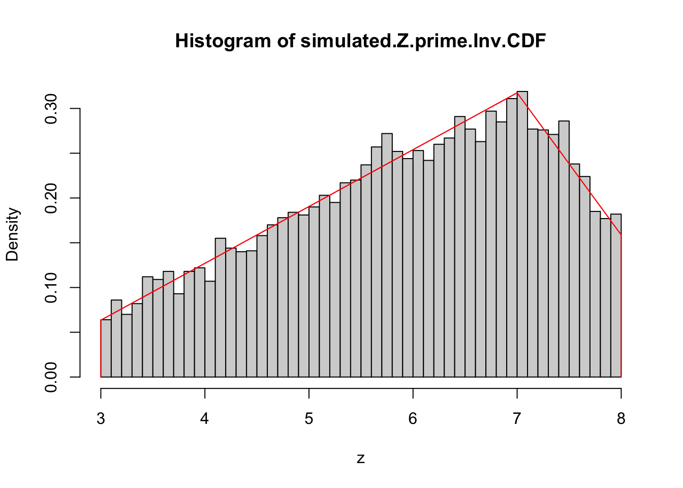
The truncated triangular PDF seems to closely fit the random sample. This is a good sign that our procedure is correct but is not enough to say for sure.
4.3.2 Trial and Error
An expression for the inverse CDF of a distribution is not always easy or possible to derive. If such is the case, we execute the following procedure. One weakness of this approach is it only works for random variables on a closed, finite interval, meaning that the likes of the normal and exponential distributions can’t be simulated reliably. Also, this is a slower approach because we can’t know how long it will take until we’ve sampled enough numbers from the distribution. Luckily, the truncated distribution requires that we simulate within an interval and the expected value of iterations until we reach the desired sample size is its minimum the way it is implemented in our code.
Find a constant function that is always greater than the PDF you are trying to simulate. The closer this constant is to being the max of the PDF the better.
Take a uniform random number and transform it on the interval of the domain of your PDF.
Take the next random uniform number, and transform it so it falls between 0 and the constant you found on step one.
Evaluate if the transformed value in step three is less than or equal to the PDF evaluated on the transformed value from step two.
If the condition in step four is met, add the transformed value from step 2 to your sample of the PDF.
Repeat steps two through five until you have gathered your goal sample size.
Let’s see this procedure implemented programatically.
## Simulate 10000 instances of a random variable with f(x) = truncated triangular by trial and error.
simulated.Z.prime.t.and.e <- rep(0, 10000)
success.count <- 0
## Stop once we've achieved 10000 succesful numbers
while (success.count < 10000) {
  ## Step 2
  u.1 <-
    runif(
      n = 1,
      min = my.trun.tri.dist$trun.tri.lower,
      max = my.trun.tri.dist$trun.tri.upper
    )
  ## Step 3
  u.2 <-
    runif(
      n = 1,
      min = 0,
      max = my.trun.tri.dist$pdf(my.trun.tri.dist$trun.tri.mode)
    )
  ## Step 4
  if (u.2 <= my.trun.tri.dist$pdf(u.1)) {
    # Step 5
    success.count <- success.count + 1
    simulated.Z.prime.t.and.e[success.count] <- u.1
  }
}
In the case of the truncated triangular PDF we know it reaches its maximum when evaluated on its mode, meaning we can take the value \(h(mode)\) as the constant of step 1.
Again, let’s plot these results to see how we did.
## Plot and describe the first simulation with many bins
hist(simulated.Z.prime.t.and.e,
     xlab = "z",
     breaks = (my.trun.tri.dist$trun.tri.upper - my.trun.tri.dist$trun.tri.lower) * 10,
     freq = FALSE)

plot.function(
  function(z) {sapply(z, my.trun.tri.dist$pdf)},
  from = 2.99999,
  to = 8.0001,
  n = 100000,
  col = "red",
  add = TRUE
)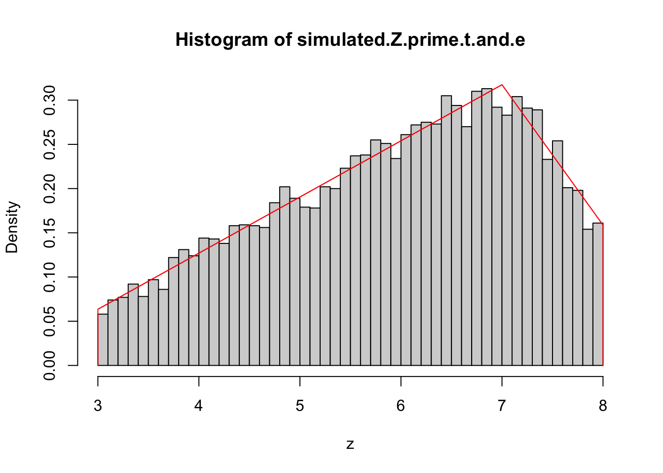
Once again, the distribution closely ressembles the sampled data. Next, we will look into testing the hypothesis that the sample matches the distribution.
Whichever method is fine for simulating or sampling PDFs, but know that each has its benefits. You would use the inverse CDF ideally on all scenarios as it is easy to implement, given an inverse CDF, but if such is not available to you or there is no interest in deriving one, the slower simulation by trial and error would still prove reliable.