2 Triangular Distribution
2.1 Distributions
Probability density functions describe how likely it is for a continuous random variable \(Y\) to fall within some region of its domain. For any single point the probability is cero but at intervals we can calculate the integral of the PDF and find the corresponding probability. Consider the following conventions:
Let \(Y\) be a random variable with distribution \(f(y)\)
This way of defining random variables lets on some basic information about how it may behave but is lengthy and unnecessary.
Let \(Y\sim f(y)\)
Much better.
Let \(Y\sim f(y) = \frac{e^{-\frac{1}{2}\left( \frac{y-\mu}{\sigma}\right)^{2}}}{\sigma \sqrt{2\pi}}\)
A PDF will sometimes be defined for the entire real number line in a single expression like the ubiquitous normal distribution, while others require you to write piecewise functions such as the triangular distribution.
Let \(Y\sim Norm(\mu, \sigma^{2})\) and \(X\sim Triangular(L,U,M)\)
We use a shorthand notation for widely used distributions that would usually take too much effort to remember or write out.
2.2 Triangular PDF
The triangular distribution specifically has the following PDF.
\[ f(x)= \begin{cases} \frac{2(x-L)}{(U-L)(M-L)}\quad&(L\leq x<M)\\ \frac{2(U-x)}{(U-L)(U-M)}\quad&(M\leq x\leq U)\\ \end{cases} \]
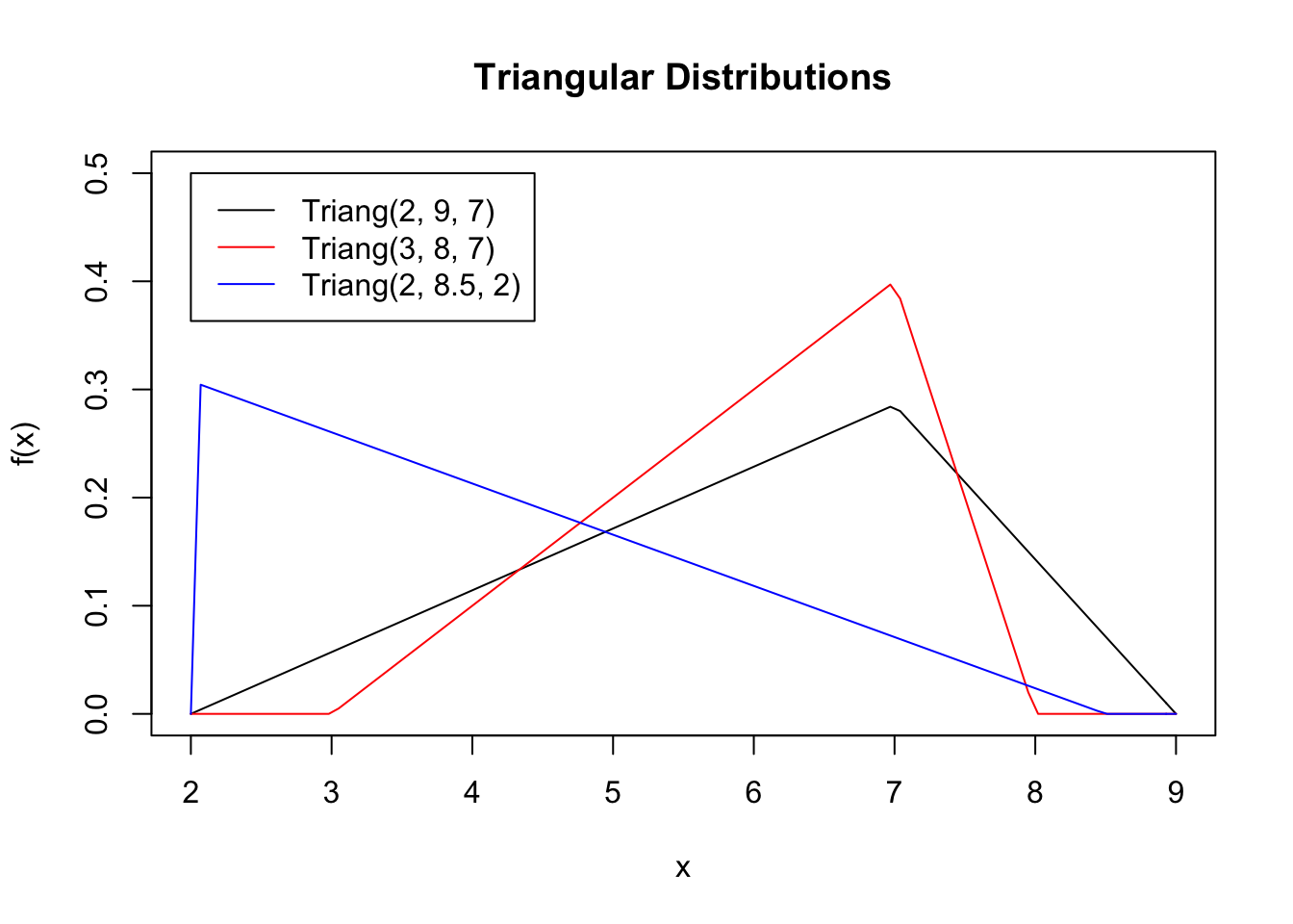
Though complicated at first sight, it really just describes two lines that form a triangle with the \(x\) axis. \(L\) and \(U\) stand for the lower and upper values that delimit the distribution and \(M\) is the mode. The function is explicit for when its value is different from cero, meaning we exclude the self-evident conditions for which it’s cero.
Let’s start writing some code and see some plots of this distribution in action.
triangular.distribution <- function(x, L, U, M) {
  if (x < L) {
    result <- 0
  } else if (x < M) {
    result <- 2 * (x - L) / ((U - L) * (M - L))
  } else if (x == M) {
    result <- 2 / (U - L)
  } else if (x <= U) {
    result <- 2 * (U - x) / ((U - L) * (U - M))
  } else if (U < x) {
    result <- 0
  }
  return(result)
}
This function takes some x and evaluates the triangular PDF defined by \(L\), \(U\), and \(M\) on it.
Because of the nature of the plot.function() method, we must make our function compatible with vectors, meaning that passing a vector as its x parameter would apply the function to every element in it. Notice the .... This just means that any subsequent parameters get passed to the underlying triangular.distribution() function.
plot.function(
  function(x) {triangular.distribution.vectorized(x, 2, 9, 7)},
  from = 2,
  to = 9,
  main = "Triangular Distributions",
  ylab = "f(x)",
  ylim = c(0, 0.5)
)

## Additional plots get included in the first rather than into a new canvas
## when the `add` parameter is set to TRUE.
plot.function(
  function(x) {triangular.distribution.vectorized(x, 3, 8, 7)},
  from = 2,
  to = 9,
  col = "red",
  add = TRUE
)

plot.function(
  function(x) {triangular.distribution.vectorized(x, 2, 8.5, 2)},
  from = 1.9999999,
  to = 9,
  col = "blue",
  add = TRUE
)

## Let's also include a legend so we can distinguish all three distributions.
legend(
  x = 2,
  y = 0.5,
  legend = c("Triang(2, 9, 7)", "Triang(3, 8, 7)", "Triang(2, 8.5, 2)"),
  col = c("black", "red", "blue"),
  lty = 1
)
Notice how our distributions take the shape of a triangle when \(x\) falls within the interval of \(L\) and \(U\) but is cero everywhere else.
2.3 Triangular CDF
The PDF alone won’t do us much good, considering how we still need to calculate probabilities somehow (remember, at any point the probability of a continuous random variable is 0).
Let us define the CDF as the probability that our random variable \(X\) is smaller than some value \(x\). Or in mathematical notation:
\[ F(x) = P\left( X \leq x \right) = \int_{-\infty}^{x}f(t)dt = \int_{L}^{x}f(t)dt \]
The PDF is defined by two continuous lines and so it follows that we could compute the integral from negative infinity to some \(x\) to be:
\[ F(x)= \begin{cases} \frac{(x-L)^{2}}{(U-L)(M-L)}\quad&(L\leq x<M)\\ 1 - \frac{(U-x)^{2}}{(U-L)(U-M)}\quad&(M\leq x\leq U)\\ 1 \quad& (U < x)\\ \end{cases} \]
We can now implement this in R in similar fashion to our PDF.
cumulative.triangular.distribution <- function(x, L, U, M) {
  if (x < L) {
    result <- 0
  } else if (x <= M) {
    result <- (x - L) ^ 2 / ((U - L) * (M - L))
  } else if (x < U) {
    result <- 1 - (U - x) ^ 2 / ((U - L) * (U - M))
  } else if (U <= x) {
    result <- 1
  }
  return(result)
}

cumulative.triangular.distribution.vectorized <- function(x, ...) {
    sapply(x, cumulative.triangular.distribution, ...)
}
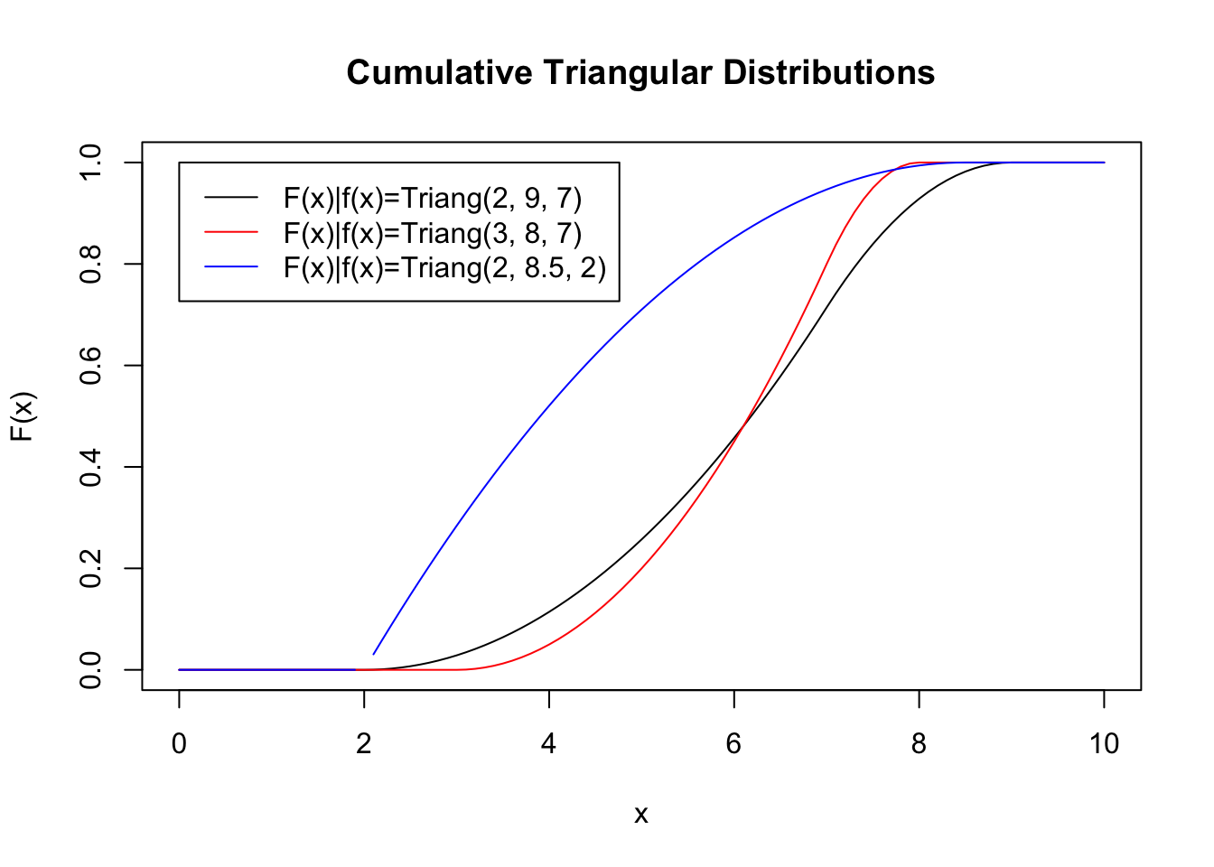
The code for the plots also shouldn’t change much. No change has been made to the parameters of each distribution.
plot.function(
  function(x) {cumulative.triangular.distribution.vectorized(x, 2, 9, 7)},
  from = 0,
  to = 10,
  main = "Cumulative Triangular Distributions",
  ylab = "F(x)",
  ylim = c(0, 1)
)

plot.function(
  function(x) {cumulative.triangular.distribution.vectorized(x, 3, 8, 7)},
  from = 0,
  to = 10,
  col = "red",
  add = TRUE
)

plot.function(
  function(x) {cumulative.triangular.distribution.vectorized(x, 2, 8.5, 2)},
  from = 0,
  to = 10,
  col = "blue",
  add = TRUE
)

legend(
  x = 0,
  y = 1,
  legend = c("F(x)|f(x)=Triang(2, 9, 7)", "F(x)|f(x)=Triang(3, 8, 7)", "F(x)|f(x)=Triang(2, 8.5, 2)"),
  col = c("black", "red", "blue"),
  lty = 1
)
Notice how the cumulative distribution approaches and becomes one very quickly. This makes sense considering that, because of the bounds of the domain of the triangular distribution, \(X\) is guaranteed to be smaller than \(U\), at which point the probability is one.
2.4 Inverse Triangular CDF
What if we already had a probability in mind but wanted to find the matching \(x\)? Well, in that case, we would need to calculate an inverse CDF. Given some probability \(p\), what \(x\) delimits \(X\) such that \(p\) is \(P(X\leq x)\).
Or in other words, find \(g\) such that:
\[ g(p) = F^{-1}(p) = F^{-1}(F(x)) = x \]
The proceure for finding the inverse of an equation of a parabola is very straight forward. The following is the inverse CDF of the triangular distribution.
\[ F^{-1}(p) = \begin{cases} L + \sqrt{(M-L)(U-L)p} \quad& (0 \leq p < \frac{M-L}{U-L})\\ U - \sqrt{(U-L)(U-M)(1-p)} \quad& (1 \geq p \geq \frac{M-L}{U-L})\\ \end{cases} \]
No plots for this one considering how it just mirrors the regular CDF over the \(y=x\) line.
inverse.cumulative.triangular.distribution <- function(p, L, U, M) {
  if (p < (M - L) / (U - L)) {
    result <- L + sqrt(max(0, (M - L) * (U - L) * p))
  } else if (p >= (M - L) / (U - L)) {
    result <- U - sqrt(max(0, (U - L) * (U - M) * (1 - p)))
  }
  return(result)
}
Notice how we artificially coerce anything within the square root to be positive, with max(0, (M - L) * (U - L) * p) for example. We do this because small rounding errors can cause issues by approximating positive values close to cero or exactly cero to a negative number whereas the square root operator is only defined for positive real numbers (Ignore complex and imaginary numbers for now).
2.5 Measures of Central Tendency and Spread
These descriptive statistics can easily be derived from the PDF and CDF. We’ll spare you the math, but keep the following in mind for their implementation in R.
2.5.1 Mean
The expected value of a random variable \(X\).
\[ E(X) = \mu = \int_{-\infty}^{\infty}xf(x)dx = \int_{L}^{U}xf(x)dx = \frac{L+U+M}{3} \]
2.5.2 Median
Value \(x\) such that the probability that a random variable \(X\) be smaller is 0.5.
\[ \text{Median(X)} = F^{-1}(0.5) = \begin{cases} L + \sqrt{\frac{(U-L)(M-L)}{2}} \quad& (M \geq \frac{L+U}{2})\\ U - \sqrt{\frac{(U-L)(U-M)}{2}} \quad& (M \leq \frac{L+U}{2})\\ \end{cases} \]
2.5.3 Mode
Value of a random variable \(X\) for which \(f(x)\) is at its maximum.
\[ \text{Mode(X)} = M \]
2.5.4 Variance
Measure of spread of the distribution with respect to the mean.
\[ \text{Var(X)} = \sigma^{2} = \int_{-\infty}^{\infty}x^{2}f(x)dx - \mu^{2} = \int_{L}^{U}x^{2}f(x)dx - \mu^{2} = \frac{L^{2} + U^{2} + M^{2} - LU - LM - UM}{18} \]
2.6 An Object to Hold These Properties
Knowing how to compute these quintessential properties of the trinagular distribution, it would make sense to build them into an object to be called on demand. Luckily, all we need is a constructor function that implements these procedures and computations and returns them in a variable that can hold multiple items of different class (a list). Consider the following constructor function that, when called, stores all explored functions and values into a list and returns it.
## Returns a function that returns a list with each of its elements defined as functions or vectors of one
## element that describe aspects of a triangular distribution
## (pdf, cdf, inverse cdf, mean, median, mode, upper bound, lower bound, variance)
generate.triangular <- function(L, U, M) {

  ## Create a function that returns the pdf of the triangular, given some x.
  pdf <- function(x) {
    if (x < L) {
      result <- 0
    } else if (x < M) {
      result <- 2 * (x - L) / ((U - L) * (M - L))
    } else if (x == M) {
      result <- 2 / (U - L)
    } else if (x <= U) {
      result <- 2 * (U - x) / ((U - L) * (U - M))
    } else if (U < x) {
      result <- 0
    }
    return(result)
  }

  ## Create a function that returns the cdf of the triangular, given some x.
  cdf <- function(x) {
    if (x <= L) {
      result <- 0
    } else if (x <= M) {
      result <- ((x - L) ^ 2) / ((U - L) * (M - L))
    } else if (x < U) {
      result <- 1 - ((U - x) ^ 2) / ((U - L) * (U - M))
    } else if (U <= x) {
      result <- 1
    }
    return(result)
  }

  ## Create a function that returns the inverse cdf of the triangular, given some probability p.
  inverse.cdf <- function(p) {
    if (p < (M - L) / (U - L)) {
      result <- L + sqrt(max(0, (M - L) * (U - L) * p))
    } else if (p >= (M - L) / (U - L)) {
      result <- U - sqrt(max(0, (U - L) * (U - M) * (1 - p)))
    }
    return(result)
  }

  ## Create a vector of length 1 that describes the mean of the distribution
  tri.mean <- (L + U + M) / 3

  ## Create a vector of length 1 that describes the median of the distribution
  tri.median <- inverse.cdf(0.5)

  ## Create a vector of length 1 that describes the mode of the distribution
  tri.mode <- M

  ## Create a vector of length 1 that describes the upper bound of the distribution's domain
  tri.upper <- U

  ## Create a vector of length 1 that describes the lower bound of the distribution's domain
  tri.lower <- L

  ## Create a vector of length 1 that describes the variance of the distribution
  tri.var <-
    ((L ^ 2) + (U ^ 2) + (M ^ 2) - L * U - L * M - U * M) / 18

  ## Build the list and return it. This list contains all major properties of the triangular distribution
  return(
    list(
      pdf = pdf,
      cdf = cdf,
      inverse.cdf = inverse.cdf,
      tri.mean = tri.mean,
      tri.median = tri.median,
      tri.mode = tri.mode,
      tri.upper = tri.upper,
      tri.lower = tri.lower,
      tri.var = tri.var
    )
  )
}